Before you begin
- Labs create a Google Cloud project and resources for a fixed time
- Labs have a time limit and no pause feature. If you end the lab, you'll have to restart from the beginning.
- On the top left of your screen, click Start lab to begin

Load Data into Portfolio, Category, and Product Tables
/ 30
Load Data into Campaigns Table
/ 20
Add column to Category Table
/ 20
Add secondary index to Category table
/ 30
Load Data into Portfolio, Category, and Product Tables
/ 30
Load Data into Campaigns Table
/ 20
Add column to Category Table
/ 20
Add secondary index to Category table
/ 30


Spanner is Google's fully managed, horizontally scalable relational database service. Customers in financial services, gaming, retail, and many other industries trust it to run their most demanding workloads, where consistency and availability at scale are critical.
In this lab, you review schema-related features of Spanner and apply those to a Banking Operations database. You also review the methods and rules by which Spanner creates query plans.
In this lab, you learn how to modify schema-related attributes of a Spanner instance:
Read these instructions. Labs are timed and you cannot pause them. The timer, which starts when you click Start Lab, shows how long Google Cloud resources are made available to you.
This hands-on lab lets you do the lab activities in a real cloud environment, not in a simulation or demo environment. It does so by giving you new, temporary credentials you use to sign in and access Google Cloud for the duration of the lab.
To complete this lab, you need:
Click the Start Lab button. If you need to pay for the lab, a dialog opens for you to select your payment method. On the right is the Lab setup and access panel with the following:
Note that the lab timer is located near the top of the page, showing the remaining time.
Click Open Google Cloud console (or right-click and select Open Link in Incognito Window if you are running the Chrome browser).
The lab spins up resources, and then opens another tab that shows the Sign in page.
Tip: Arrange the tabs in separate windows, side-by-side.
If necessary, copy the Username below and paste it into the Sign in dialog.
You can also find the Username in the Lab setup and access panel.
Click Next.
Copy the Password below and paste it into the Welcome dialog.
You can also find the Password in the Lab setup and access panel.
Click Next.
Click through the subsequent pages:
After a few moments, the Google Cloud console opens in this tab.

Cloud Shell is a virtual machine that is loaded with development tools. It offers a persistent 5GB home directory and runs on the Google Cloud. Cloud Shell provides command-line access to your Google Cloud resources.
Click Activate Cloud Shell 
Click through the following windows:
When you are connected, you are already authenticated, and the project is set to your Project_ID,
gcloud is the command-line tool for Google Cloud. It comes pre-installed on Cloud Shell and supports tab-completion.
Output:
Output:
gcloud, in Google Cloud, refer to the gcloud CLI overview guide.
To help you move quickly through this lab, the lab environment automatically creates a Spanner instance, database, and tables for you.
Here are the resource details for your reference:
| Item | Name | Details |
|---|---|---|
| Spanner instance | banking-ops-instance |
Project-level instance |
| Spanner database | banking-ops-db |
Instance-specific database |
| Table | Portfolio |
Contains top-level bank offerings |
| Table | Category |
Contains second-tier bank offering groupings |
| Table | Product |
Contains specific line-item bank offerings |
| Table | Campaigns |
Contains details on marketing initiatives |
The banking-ops-db database starts with empty tables. Complete the following steps to load data into three of the tables (Portfolio, Category, and Product).
In the Google Cloud console, on the Navigation menu (
Click banking-ops-instance to explore its databases.
Click banking-ops-db and scroll down to Tables to view the four existing tables.
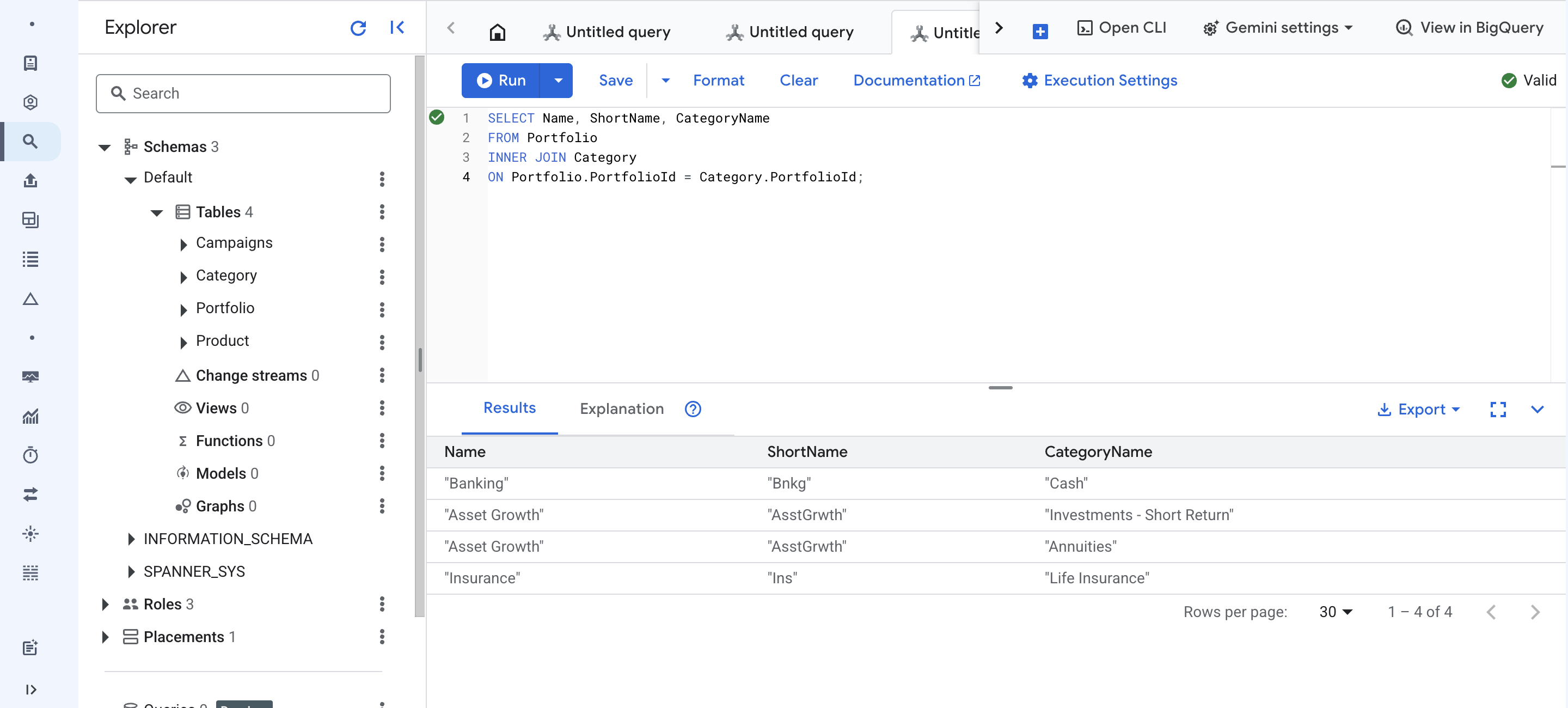
In the navigation pane, click Spanner Studio, and then click New SQL editor tab (+) to open a new SQL editor.
In the SQL editor, paste the following INSERT statement to load the Portfolio table, and then click Run (Spanner runs each row insertion in succession):
The Results pane displays the status of the statement. A check mark indicates that the statement completed successfully, and the Portfolio table now has three rows.
Click Clear in the SQL editor toolbar.
Paste the following INSERT statement to load the Category table, and then click Run:
The Results pane displays the status of the INSERT operation. A check mark indicates that the statement completed successfully, and the Category table now has four rows.
Click Clear in the SQL editor toolbar.
Paste the following INSERT statement to load the Product table, and then click Run:
The Results pane displays the status of the INSERT operation. A check mark indicates that the statement completed successfully, and the Product table now has nine rows.
Click Check my progress to verify the objective.
In the next several steps, you use the Spanner client library for Python.
snippets.py file contains multiple Spanner DDL, DML, and DCL functions that you use as helper code during this lab. Run snippets.py with the insert_data argument to populate the Campaigns table:Click Check my progress to verify the objective.
You can use the query_data() function in snippets.py to query your database. In this task, you run it to confirm that the script loaded data into the Campaigns table. You do not need to modify the following reference code:
snippets.py with the query_data argument to query the Campaigns table:The output resembles the following:
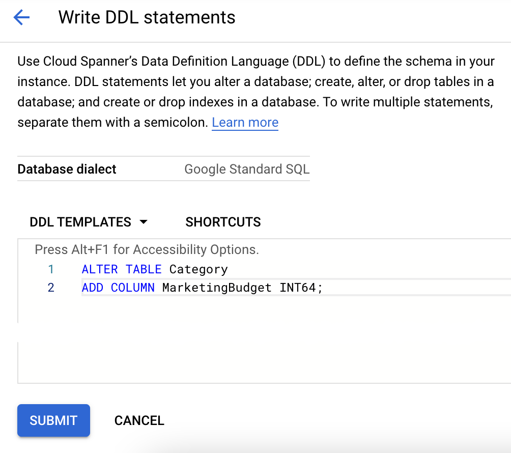
As a database administrator (DBA), you need to add a new column named MarketingBudget to the Category table. Adding a new column to an existing table requires an update to your database schema. Spanner supports schema updates to a database while the database continues to serve traffic. Schema updates do not require taking the database offline and do not lock entire tables or columns; you can continue reading and writing data to the database during the schema update.
The update_ddl() method of the Database class modifies the schema.
Use the add_column() function in snippets.py, which calls this method. You do not need to modify the following reference code:
snippets.py with the add_column argument:Click Check my progress to verify the objective.
The following command performs the same schema update that you ran with Python:
The following code writes data to the new column. It sets MarketingBudget to 100000 for the row with a CategoryId of 1 and a PortfolioId of 1, and sets it to 500000 for the row with a CategoryId of 3 and a PortfolioId of 2. You do not need to modify the following reference code:
snippets.py with the update_data argument:snippets.py with the query_data_with_new_column argument:The output is as follows:
Suppose you want to fetch all rows from the Category table that have CategoryName values in a certain range. You could read all values from the CategoryName column using a SQL statement or a read call, and then discard the rows that don't meet the criteria, but doing this full table scan is expensive, especially for tables with many rows. Instead, you can speed up the retrieval of rows when searching by non-primary key columns by creating a secondary index on the table.
Adding a secondary index to an existing table requires a schema update. Like other schema updates, Spanner supports adding an index while the database continues to serve traffic. Spanner populates the index with data (also known as a backfill) automatically in the background. Backfills might take several minutes to complete, but you don't have to take the database offline or avoid writing to certain tables or columns during this process.
Use the add_index() function to create a secondary index. You do not need to modify the following reference code:
snippets.py with the add_index argument:Click Check my progress to verify the objective.
To read data using the index, call the read() method with the index specified. You do not need to modify the following reference code:
snippets.py with the read_data_with_index argument:The output is as follows:
Notice that the preceding read example did not read the MarketingBudget column. Spanner's read interface does not support joining an index with a data table to look up values that the index does not store.
To bypass this restriction, create an alternate definition of the CategoryByCategoryName index that stores a copy of MarketingBudget in the index.
Use the update_ddl() method of the Database class to add an index with a STORING clause. You do not need to modify the following reference code:
snippets.py with the add_storing_index argument:Now you can run a read operation that fetches the CategoryId, CategoryName, and MarketingBudget columns using the CategoryByCategoryName2 index. You do not need to modify the following reference code:
snippets.py with the read_data_with_storing_index argument:The output is as follows:
In this section, you explore Spanner query plans.
The result resembles the following:
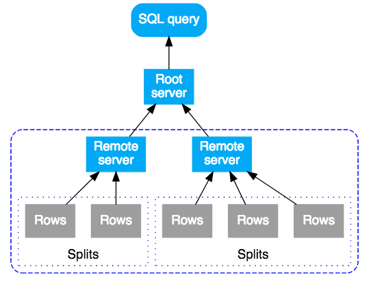
Spanner first compiles a SQL query into an execution plan and sends it to an initial root server for execution. Spanner chooses the root server to minimize the number of hops required to reach the queried data. The root server then performs the following actions:
Remote servers that receive a subplan act as the "root" server for their subplan, following the same model as the top-most root server. The result is a tree of remote executions. Conceptually, query execution flows from top to bottom, and the servers return query results from bottom to top. The following diagram shows this pattern:
Now examine the query plan for an aggregate query.
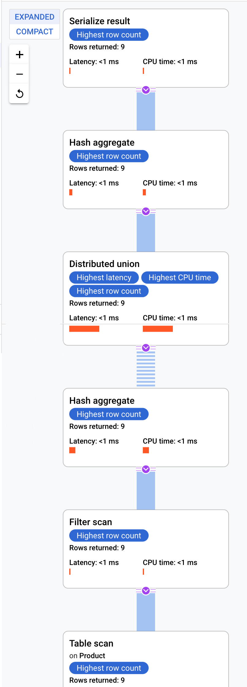
Spanner sends the execution plan to a root server that coordinates the query execution and performs the remote distribution of subplans.
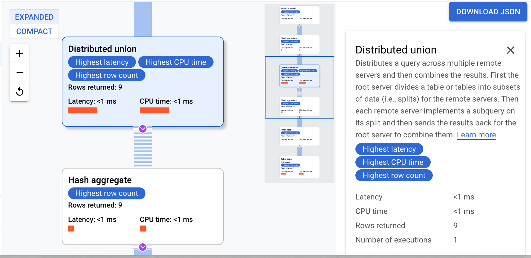
This execution plan starts with a serialization step that orders all returned values. Next, the plan runs an initial hash aggregate operator to calculate preliminary results, and then runs a distributed union that distributes subplans to remote servers whose splits satisfy ProductId < 100. The distributed union sends results to a final hash aggregate operator. The aggregate operator performs the COUNT aggregation by ProductId and returns results to a serialize result operator. Finally, the plan runs a scan to order the returned results.
The query plan resembles the following:
Spanner physically stores interleaved tables with the rows of their related tables co-located. A join between interleaved tables is known as a co-located join. Co-located joins can offer performance benefits over joins that require indexes or back joins.
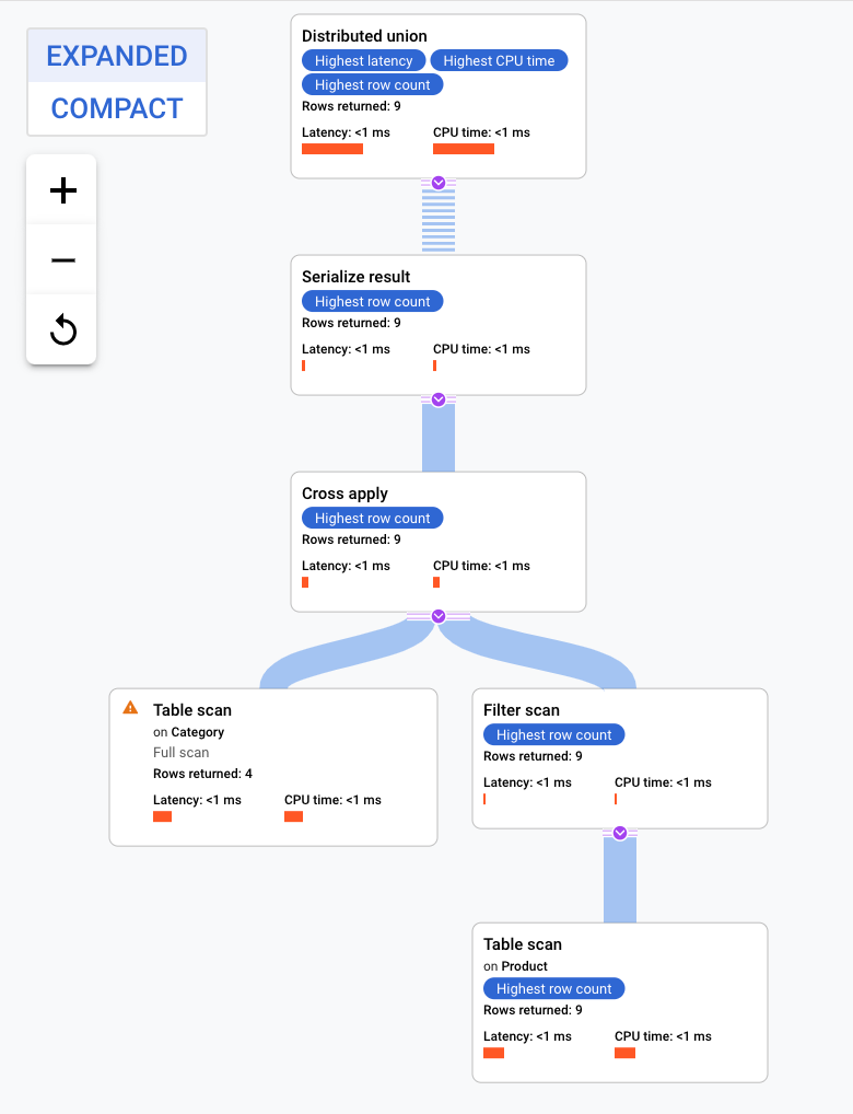
This execution plan starts with a distributed union, which distributes subplans to remote servers that have splits of the Category table. Because Product is an interleaved table of Category, each remote server can execute the entire subplan locally without requiring a join across different servers.
The subplans contain a cross apply. Each cross apply performs a table scan on the Category table to retrieve PortfolioId, CategoryId, and CategoryName. The cross apply then maps output from the table scan to output from an index scan on the CategoryByCategoryName index, subject to a filter of the PortfolioId in the index matching the PortfolioId from the table scan output. Each cross apply sends its results to a serialize result operator that serializes the CategoryName and ProductName data and returns results to the local distributed unions. The distributed union aggregates results from the local distributed unions and returns them as the query result.
You now have a solid understanding of the schema-related features of Spanner and the methods by which Spanner creates query plans.
...helps you make the most of Google Cloud technologies. Our classes include technical skills and best practices to help you get up to speed quickly and continue your learning journey. We offer fundamental to advanced level training, with on-demand, live, and virtual options to suit your busy schedule. Certifications help you validate and prove your skill and expertise in Google Cloud technologies.
Copyright 2026 Google LLC. All rights reserved. Google and the Google logo are trademarks of Google LLC. All other company and product names may be trademarks of the respective companies with which they are associated.


This content is not currently available
We can notify you via email when it becomes available

Great!
We can contact you via email if it becomes available

One lab at a time
Confirm to end all existing labs and start this one