


Before you begin
- Labs create a Google Cloud project and resources for a fixed time
- Labs have a time limit and no pause feature. If you end the lab, you'll have to restart from the beginning.
- On the top left of your screen, click Start lab to begin
Setup the data environment
/ 10
Run your pipeline
/ 10
Generate lag-less streaming input
/ 10
In this lab, you take many of the concepts introduced in a batch context and apply them in a streaming context to create a pipeline similar to BatchMinuteTrafficPipeline, but which operates in real time. The finished pipeline will first read JSON messages from Pub/Sub and parse those messages before branching. One branch writes some raw data to BigQuery and takes note of event and processing time. The other branch windows and aggregates the data and then writes the results to BigQuery.
You will build the following pipeline:
For each lab, you get a new Google Cloud project and set of resources for a fixed time at no cost.
Sign in to Qwiklabs using an incognito window.
Note the lab's access time (for example, 1:15:00), and make sure you can finish within that time.
There is no pause feature. You can restart if needed, but you have to start at the beginning.
When ready, click Start lab.
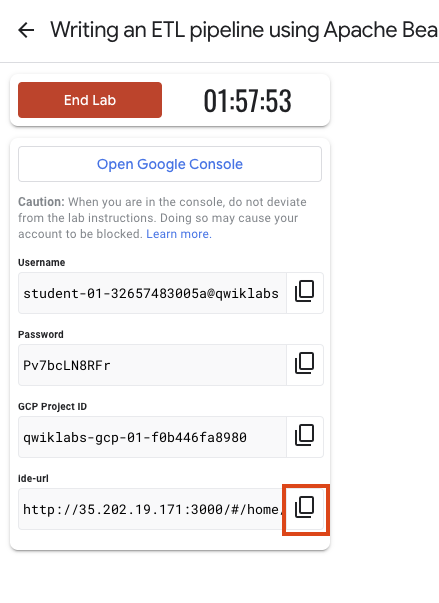
Note your lab credentials (Username and Password). You will use them to sign in to the Google Cloud Console.
Click Open Google Console.
Click Use another account and copy/paste credentials for this lab into the prompts.
If you use other credentials, you'll receive errors or incur charges.
Accept the terms and skip the recovery resource page.
Google Cloud Shell is a virtual machine that is loaded with development tools. It offers a persistent 5GB home directory and runs on the Google Cloud.
Google Cloud Shell provides command-line access to your Google Cloud resources.
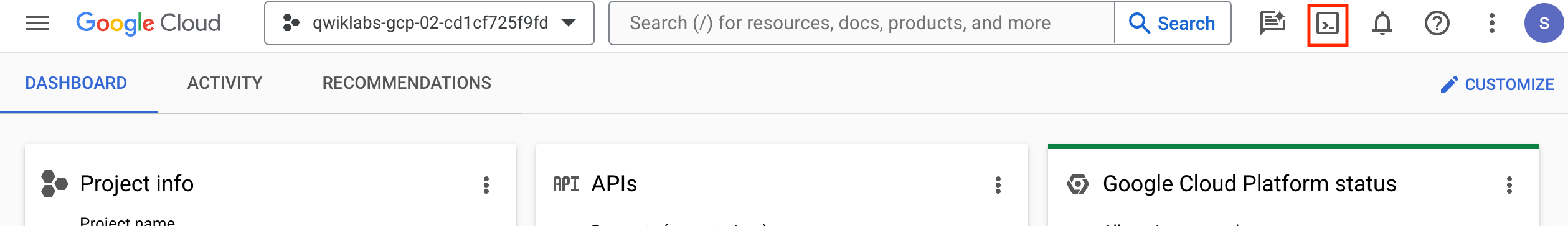
In Cloud console, on the top right toolbar, click the Open Cloud Shell button.
Click Continue.
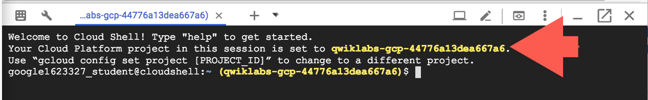
It takes a few moments to provision and connect to the environment. When you are connected, you are already authenticated, and the project is set to your PROJECT_ID. For example:
gcloud is the command-line tool for Google Cloud. It comes pre-installed on Cloud Shell and supports tab-completion.
Output:
Example output:
Output:
Example output:
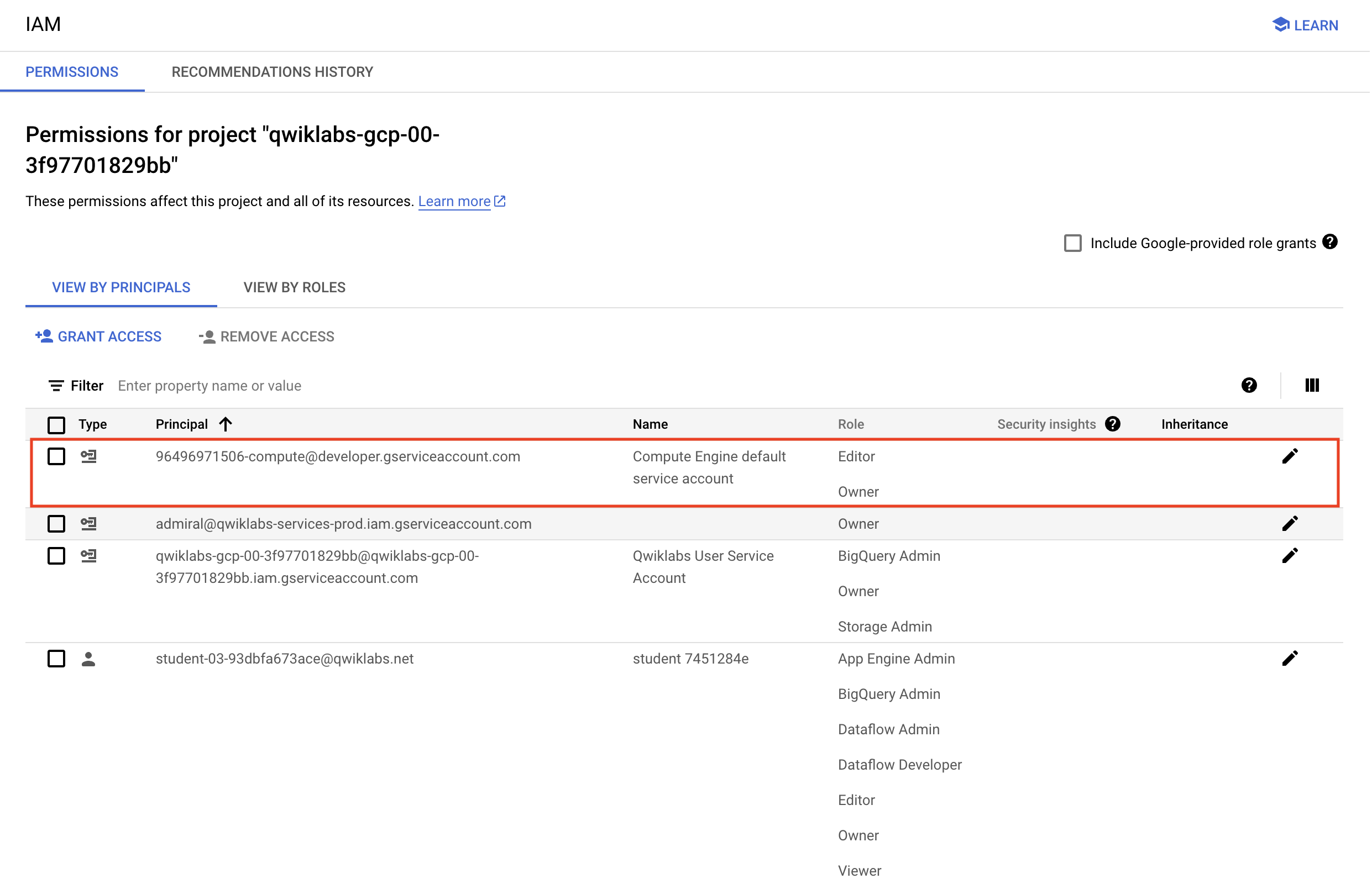
Before you begin your work on Google Cloud, you need to ensure that your project has the correct permissions within Identity and Access Management (IAM).
In the Google Cloud console, on the Navigation menu (
Confirm that the default compute Service Account {project-number}-compute@developer.gserviceaccount.com is present and has the editor role assigned. The account prefix is the project number, which you can find on Navigation menu > Cloud Overview > Dashboard.
editor role, follow the steps below to assign the required role.729328892908).{project-number} with your project number.For the purposes of this lab, you will mainly be using a Theia Web IDE hosted on Google Compute Engine. It has the lab repo pre-cloned. There is java langauge server support, as well as a terminal for programmatic access to Google Cloud APIs via the gcloud command line tool, similar to Cloud Shell.
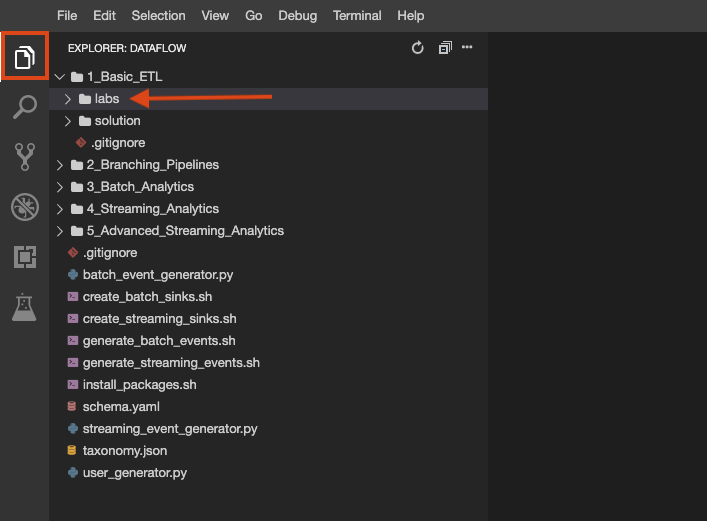
The lab repo has been cloned to your environment. Each lab is divided into a labs folder with code to be completed by you, and a solution folder with a fully workable example to reference if you get stuck.
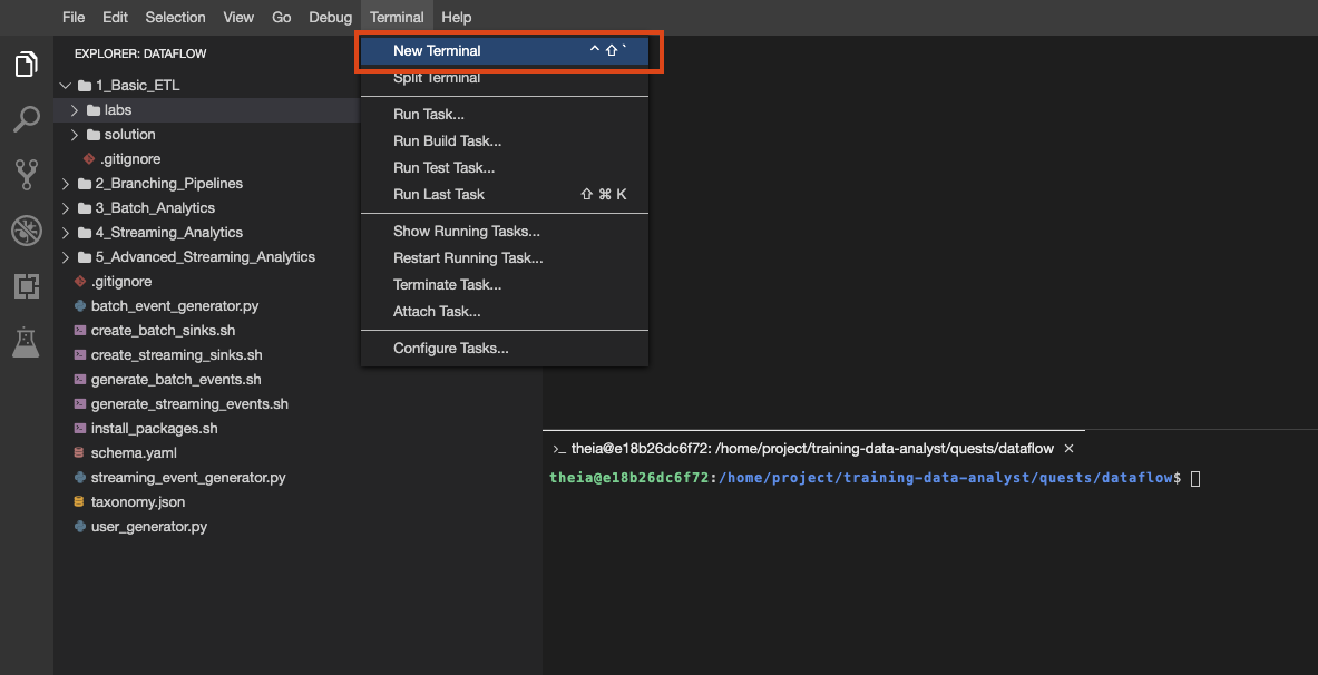
File Explorer button to look:You can also create multiple terminals in this environment, just as you would with cloud shell:
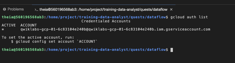
You can see with by running gcloud auth list on the terminal that you're logged in as a provided service account, which has the exact same permissions are your lab user account:
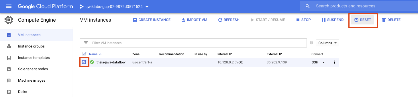
If at any point your environment stops working, you can try resetting the VM hosting your IDE from the GCE console like this:
Click Check my progress to verify the objective.
In previous labs, you used TextIO.read() to read from Google Cloud Storage. In this lab, instead of Google Cloud Storage, you use Pub/Sub. Pub/Sub is a fully managed real-time messaging service that allows publishers to send messages to a "topic," to which subscribers can subscribe via a "subscription."
The pipeline you create subscribes to a topic called my_topic that you just created via create_streaming_sinks.sh script. In a production situation, this topic will often be created by the publishing team. You can view it in the Pub/Sub portion of the console.
To read from Pub/Sub using Apache Beam’s IO connectors, open the file StreamingMinuteTrafficPipeline.java and add a transform to the pipeline that uses the PubsubIO.readStrings() function. This function returns an instance of PubsubIO.Read, which has a method for specifying the source topic as well as the timestamp attribute. Note that there is already a command-line option for the Pub/Sub topic name. Set the timestamp attribute to “timestamp”, which corresponds to an attribute that will be added to each Pub/Sub message. In the event that message publication time is sufficient, this step would be unnecessary.
To complete this task, add a transform that reads from the Pub/Sub topic specified by the inputTopic command-line parameter. Then, use the provided DoFn, JsonToCommonLog, to convert each JSON string into a CommonLog instance. Collect the results from this transform into a PCollection of CommonLog instances.
In the previous non-SQL lab, you implemented fixed-time windowing in order to group events by event time into mutually-exclusive windows of fixed size. Do the same thing here with the streaming inputs. Feel free to reference the previous lab's code or the solution if you get stuck.
PCollection of CommonLog data and windows elements into windows of windowDuration seconds long, with windowDuration as another command-line parameter.In the previous lab, you used the Count transform to count the number of events per window. Do the same here.
<Long> value to a <Row> value and extract the timestamp as follows:To complete this task, pass the windowed PCollection as input to a transform that counts the number of events per window.
Add an additional transform to convert the results back to a PCollection of Rows with the schema pageviewsSchema that has been provided for you.
This pipeline writes to BigQuery in two separate branches. The first branch writes the aggregated data to BigQuery. The second branch, which has already been authored for you, writes out some metadata regarding each raw event, including the event timestamp and the actual processing timestamp. Both write directly to BigQuery via streaming inserts.
Writing to BigQuery has been covered extensively in previous labs, so the basic mechanics will not be covered in depth here.
This task makes use of code that has been provided.
To complete this task:
Create a new command-line parameter called aggregateTableName for the table intended to house aggregated data.
Add a transform, as before, that writes to BigQuery and uses .useBeamSchema().
BigQueryIO.write() does not support WriteDisposition of WRITE_TRUNCATE in which the table is dropped and recreated. In this example, use WRITE_APPEND.BigQueryIO.Write will default to either streaming inserts for unbounded PCollections or batch file load jobs for bounded PCollections. Streaming inserts can be particularly useful when you want data to show up in aggregations immediately, but does incur extra charges.
In streaming use cases where you are OK with periodic batch uploads on the order of every couple minutes, you can specify this behavior via .withMethod(), and also set the frequency with .withTriggeringFrequency(org.joda.time.Duration).
Refer to the BigQueryIO.Write.Method documentation to learn more.
To complete this task:
Find the command-line parameter for the name of the table intended to house the raw data.
Examine the pipeline branch that has been authored for you already. It is capturing processing time in addition to the event time.
Click Check my progress to verify the objective.
Because this is a streaming pipeline, it subscribes to the streaming source and will await input; there is none currently. In this section, you generate data with no lag. Actual data will almost invariably contain lag. However, it is instructive to understand lag-less streaming inputs.
The code for this quest includes a script for publishing JSON events using Pub/Sub.
training-data-analyst/quests/dataflow folder.Click Check my progress to verify the objective.
You should see that the number of pageviews hovered around 100 views a minute.
Alternatively, you can use the BigQuery command-line tool as a quick way to confirm results are being written:
This query illustrates the gap between event time and processing time. However, it can be hard to see the big picture by looking at just the raw tabular data. We will use Looker Studio, a lightweight data visualization and BI engine.
This will open a new window.
Select the existing bar chart. In the right-hand panel, change the chart type to scatter chart.
In the Setup column of the panel on the right-hand side, set the following values:
The chart will transform to be a scatterplot, where all points are on the diagonal. This is because in the streaming data currently being generated, events are processed immediately after they were generated — there was no lag. If you started the data generation script quickly, i.e. before the Dataflow job was fully up and running, you may see a hockey stick, as there were messages queuing in Pub/Sub that were all processed more or less at once.
But in the real world, lag is something that pipelines need to cope with.
The streaming event script is capable of generating events with simulated lag.
This represents scenarios where there is a time delay between when the events are generated and published to Pub/Sub, for example when a mobile client goes into offline mode if a user has no service, but events are collected on the device and all published at once when the device is back online.
First, close the Looker Studio window.
Then, to turn on lag, return to the window containing IDE Terminal.
Next, stop the running script using CTRL+C in the Terminal.
Then, run the following:
The new data that arrive, which should appear on the right side of the chart, should no longer be perfect; instead, some will appear above the diagonal, indicating that they were processed after the events transpired.
Chart Type: Scatter
When you have completed your lab, click End Lab. Google Cloud Skills Boost removes the resources you’ve used and cleans the account for you.
You will be given an opportunity to rate the lab experience. Select the applicable number of stars, type a comment, and then click Submit.
The number of stars indicates the following:
You can close the dialog box if you don't want to provide feedback.
For feedback, suggestions, or corrections, please use the Support tab.
Copyright 2022 Google LLC All rights reserved. Google and the Google logo are trademarks of Google LLC. All other company and product names may be trademarks of the respective companies with which they are associated.


This content is not currently available
We will notify you via email when it becomes available

Great!
We will contact you via email if it becomes available

One lab at a time
Confirm to end all existing labs and start this one