Overview

In this lab, you:

• Write a pipeline that aggregates site traffic by user.
• Write a pipeline that aggregates site traffic by minute.
• Implement windowing on time series data.

Prerequisites

Basic familiarity with Java.

Setup and requirements

For each lab, you get a new Google Cloud project and set of resources for a fixed time at no cost.

1. Sign in to Qwiklabs using an incognito window.

2. Note the lab's access time (for example, 1:15:00), and make sure you can finish within that time.
   There is no pause feature. You can restart if needed, but you have to start at the beginning.

3. When ready, click Start lab.

4. Note your lab credentials (Username and Password). You will use them to sign in to the Google Cloud Console.

5. Click Open Google Console.

6. Click Use another account and copy/paste credentials for this lab into the prompts.
   If you use other credentials, you'll receive errors or incur charges.

7. Accept the terms and skip the recovery resource page.

Check project permissions

Before you begin your work on Google Cloud, you need to ensure that your project has the correct permissions within Identity and Access Management (IAM).

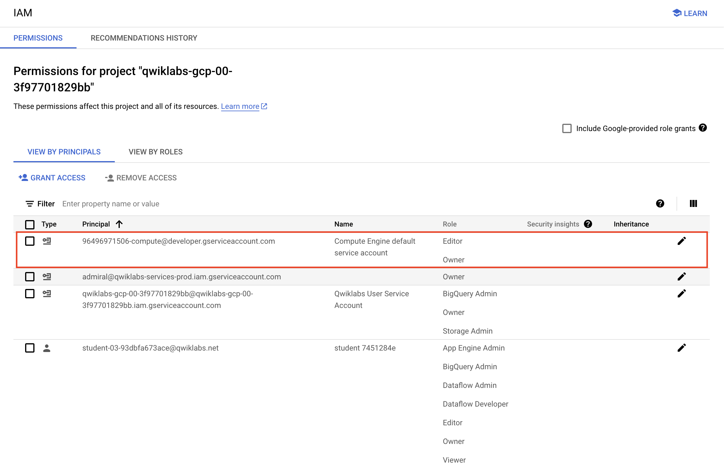
1. In the Google Cloud console, on the Navigation menu (), select IAM & Admin > IAM.

2. Confirm that the default compute Service Account {project-number}-compute@developer.gserviceaccount.com is present and has the editor role assigned. The account prefix is the project number, which you can find on Navigation menu > Cloud Overview > Dashboard.

Note: If the account is not present in IAM or does not have the editor role, follow the steps below to assign the required role.

1. In the Google Cloud console, on the Navigation menu, click Cloud Overview > Dashboard.
2. Copy the project number (e.g. 729328892908).
3. On the Navigation menu, select IAM & Admin > IAM.
4. At the top of the roles table, below View by Principals, click Grant Access.
5. For New principals, type:

{project-number}-compute@developer.gserviceaccount.com

6. Replace {project-number} with your project number.
7. For Role, select Project (or Basic) > Editor.
8. Click Save.

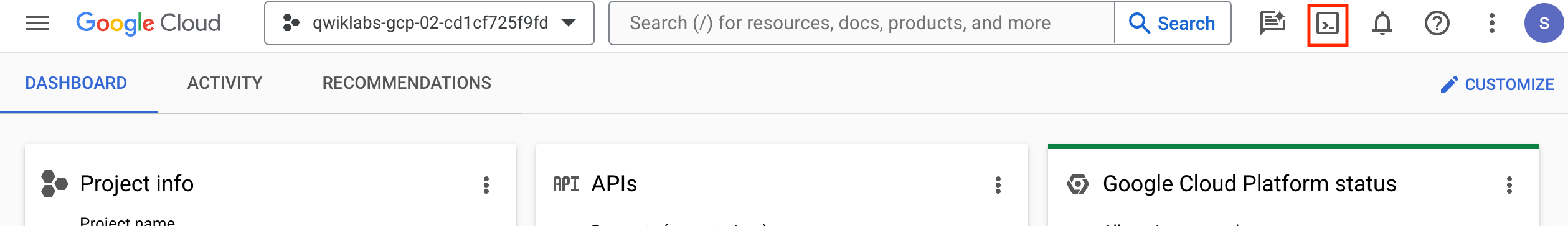
Activate Google Cloud Shell

Google Cloud Shell is a virtual machine that is loaded with development tools. It offers a persistent 5GB home directory and runs on the Google Cloud.

Google Cloud Shell provides command-line access to your Google Cloud resources.

1. In Cloud console, on the top right toolbar, click the Open Cloud Shell button.

   

2. Click Continue.

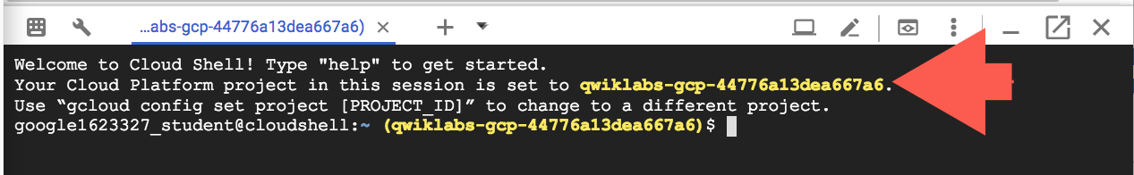
It takes a few moments to provision and connect to the environment. When you are connected, you are already authenticated, and the project is set to your PROJECT_ID. For example:

gcloud is the command-line tool for Google Cloud. It comes pre-installed on Cloud Shell and supports tab-completion.

• You can list the active account name with this command:

gcloud auth list

Output:

Credentialed accounts: - @.com (active)

Example output:

Credentialed accounts: - google1623327_student@qwiklabs.net

• You can list the project ID with this command:

gcloud config list project

Output:

[core] project =

Example output:

[core] project = qwiklabs-gcp-44776a13dea667a6 Note: Full documentation of gcloud is available in the gcloud CLI overview guide .

Setting up your IDE

For the purposes of this lab, you will mainly be using a Theia Web IDE hosted on Google Compute Engine. It has the lab repo pre-cloned. There is java langauge server support, as well as a terminal for programmatic access to Google Cloud APIs via the gcloud command line tool, similar to Cloud Shell.

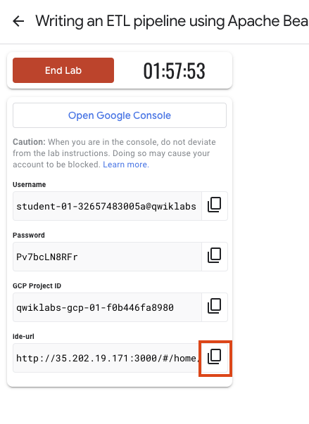
1. To access your Theia IDE, copy and paste the link shown in Google Cloud Skills Boost to a new tab.

Note: You may need to wait 3-5 minutes for the environment to be fully provisioned, even after the url appears. Until then you will see an error in the browser.

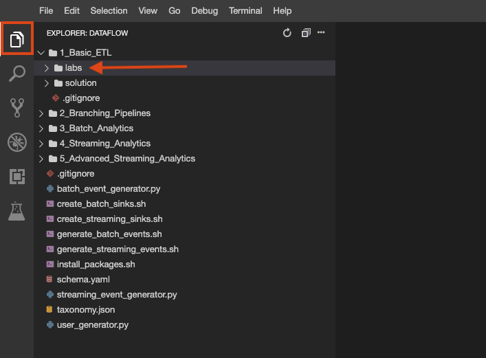
The lab repo has been cloned to your environment. Each lab is divided into a labs folder with code to be completed by you, and a solution folder with a fully workable example to reference if you get stuck.

2. Click on the File Explorer button to look:

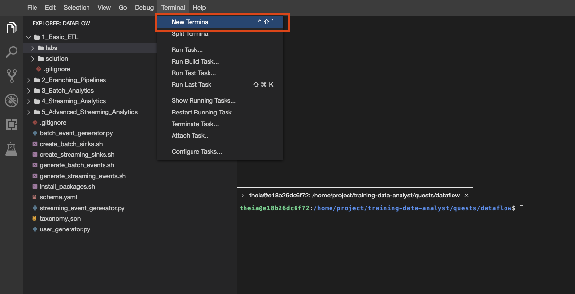
You can also create multiple terminals in this environment, just as you would with cloud shell:

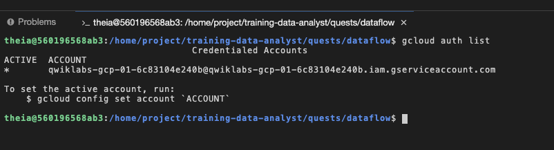
You can see with by running gcloud auth list on the terminal that you're logged in as a provided service account, which has the exact same permissions are your lab user account:

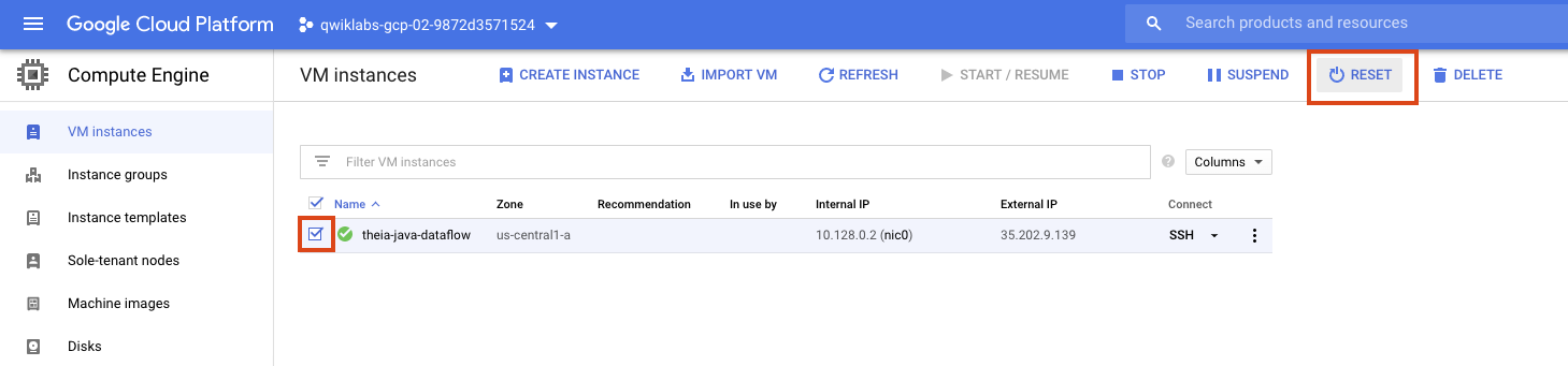
If at any point your environment stops working, you can try resetting the VM hosting your IDE from the GCE console like this:

Part 1: Aggregating site traffic by user

In this part of the lab, you write a pipeline that:

1. Reads the day’s traffic from a file in Cloud Storage.
2. Converts each event into a CommonLog object.
3. Sums the number of hits for each unique user by grouping each object by user ID and combining the values to get the total number of hits for that particular user.
4. Performs additional aggregations on each user.
5. Writes the resulting data to BigQuery.

Task 1. Generate synthetic data

As in the prior labs, the first step is to generate data for the pipeline to process. You will open the lab environment and generate the data as before:

Open the appropriate lab

• Create a new terminal in your IDE environment, if you haven't already, and copy and paste the following command:

# Change directory into the lab cd 3_Batch_Analytics/labs # Download dependencies mvn clean dependency:resolve export BASE_DIR=$(pwd)

Set up the data environment

# Create GCS buckets and BQ dataset cd $BASE_DIR/../.. source create_batch_sinks.sh # Generate event dataflow source generate_batch_events.sh # Change to the directory containing the practice version of the code cd $BASE_DIR

The script creates a file called events.json containing lines resembling the following:

{"user_id": "-6434255326544341291", "ip": "192.175.49.116", "timestamp": "2019-06-19T16:06:45.118306Z", "http_request": "\"GET eucharya.html HTTP/1.0\"", "lat": 37.751, "lng": -97.822, "http_response": 200, "user_agent": "Mozilla/5.0 (compatible; MSIE 7.0; Windows NT 5.01; Trident/5.1)", "num_bytes": 182}

It then automatically copies this file to your Google Cloud Storage bucket at gs://my-project-id/events.json.

• Navigate to Google Cloud Storage and confirm that your storage bucket contains a file called events.json.

Click Check my progress to verify the objective. Generate synthetic data

Task 2. Sum pageviews per user

1. Open up BatchUserTrafficPipeline.java in your IDE, which can be found in 3_Batch_Analytics/labs/src/main/java/com/mypackage/pipeline.

This pipeline already contains the necessary code to accept command-line options for the input path and the output table name, as well as code to read in events from Google Cloud Storage, parse those events, and write results to BigQuery. However, some important parts are missing.

2. The next step in the pipeline is to aggregate the events by each unique user_id and count pagviews for each. Any easy way to do this on Rows or objects with a Beam schema is to use the Group.byFieldNames() transform and then perform some aggregations on the resulting group. For example:

purchases.apply(Group.<MyObject>byFieldNames("userId", "address"));

will return a PCollection of rows with two fields, "key" and "values". The "key" field is itself a Row with schema <userID:STRING, address:STRING> representing every unique combination of userID and address. The "values" field is of type ITERABLE[ROW[MyObject]] containing all of the objects in that unique group.

FieldName	FieldType
key	ROW{userId:STRING, streetAddress:STRING}
values	ITERABLE[ROW[Purchase]]

3. This is most useful when you can perform aggregate calculations on this grouping and name the resulting fields, like so:

purchases.apply(Group.byFieldNames("userId") .aggregateField("itemId", Count.combineFn(), "numPurchases") .aggregateField("costCents", Sum.ofLongs(), "totalSpendCents") .aggregateField("costCents", Max.ofLongs(), "largestPurchases"));

This returns a "key" "value" Row, as opposed to "values" plural.

FieldName	FieldType
key	ROW{userId:STRING}
value	ROW{numPurchases: INT64, totalSpendCents: INT64, largestPurchases: INT64}

The Sum and Count transforms are perfect for this use. Sum and Count are examples of Combine transforms that can act on groups of data.

Note: In this example you could aggregate on any of the fields for Count.combineFn(), or even on the wildcard field *, as this transform is simply counting how many elements are in the entire group.

4. The next step in the pipeline is to aggregate events by user_id, sum the pageviews, and also calculate some additional aggregations on num_bytes, for example total user bytes.

To complete this task, add another transform to the pipeline which groups the events by user_id and then performs the relevant aggregations. Keep in mind the input, the CombineFns to use, and how you name the output fields.

Task 3. Flatten the schema

At this point, your new transform is returning a PCollection with schema <Key,Value> as already mentioned. If you run your pipeline as is, it will be written to BigQuery as two nested RECORDS, even though there is essentially only one row of values in each.

1. You can avoid this by adding a Select transform like the following:

purchases.apply(Group.byFieldNames("userId") .aggregateField("itemId", Count.combineFn(), "numPurchases") .aggregateField("costCents", Sum.ofLongs(), "totalSpendCents") .aggregateField("costCents", Max.ofLongs(), "largestPurchases")) .apply(Select.fieldNames("key.userId", "value.numPurchases", "value.totalSpendCents", "value.largestPurchases")

This will retain the relevant field names in the new flattened Schema, and remove "key" and "value".

2. To complete this task, add a Select Transform to flatten the schema of your new row.

Note: Remember to change the object hint in BigQueryIO.<CommonLog>write() to <Row> if you haven't already.

Task 4. Run your pipeline

• Return to Cloud Shell and execute the following command to run your pipeline using the Dataflow service. You can run it with DirectRunner if you're having trouble, or refer to the solution.

export PROJECT_ID=$(gcloud config get-value project) export REGION={{{ project_0.default_region | "REGION" }}} export BUCKET=gs://${PROJECT_ID} export PIPELINE_FOLDER=${BUCKET} export MAIN_CLASS_NAME=com.mypackage.pipeline.BatchUserTrafficPipeline export RUNNER=DataflowRunner export INPUT_PATH=${PIPELINE_FOLDER}/events.json export TABLE_NAME=${PROJECT_ID}:logs.user_traffic cd $BASE_DIR mvn compile exec:java \ -Dexec.mainClass=${MAIN_CLASS_NAME} \ -Dexec.cleanupDaemonThreads=false \ -Dexec.args=" \ --project=${PROJECT_ID} \ --region=${REGION} \ --stagingLocation=${PIPELINE_FOLDER}/staging \ --tempLocation=${PIPELINE_FOLDER}/temp \ --runner=${RUNNER} \ --inputPath=${INPUT_PATH} \ --tableName=${TABLE_NAME}"

Click Check my progress to verify the objective. Aggregating site traffic by user and running your pipeline

Task 5. Verify results in BigQuery

1. To complete this task, wait a few minutes for the pipeline to complete, then navigate to BigQuery and query the user_traffic table.

2. If you are curious, comment out your Select transform step and re-run the pipeline to see the resulting BigQuery schema.

Part 2: Aggregating site traffic by minute

In this part of the lab, you create a new pipeline called BatchMinuteTraffic. BatchMinuteTraffic expands on the basic batch analysis principles used in BatchUserTraffic and, instead of aggregating by users across the entire batch, aggregates by when events occurred.

• In the IDE, open up the file BatchMinuteTrafficPipeline.java inside 3_Batch_Analytics/labs/src/main/java/com/mypackage/pipeline.

Task 1. Add timestamps to each element

An unbounded source provides a timestamp for each element. Depending on your unbounded source, you may need to configure how the timestamp is extracted from the raw data stream.

However, bounded sources (such as a file from TextIO, as is used in this pipeline) do not provide timestamps.

1. You can parse the timestamp field from each record and use the WithTimestamps transform to attach the timestamps to each element in your PCollection:

PCollection<MyClass> unstamped = ...; PCollection<MyClass> stamped = unstampedLogs.apply(WithTimestamps.of((MyClass m) -> org.joda.time.Instant.parse(m.getTimestamp())));

2. To complete this task, add a transform to the pipeline that adds timestamps to each element of the pipeline.

Task 2. Window into one-minute windows

Windowing subdivides a PCollection according to the timestamps of its individual elements. Transforms that aggregate multiple elements, such as GroupByKey and Combine, work implicitly on a per-window basis — they process each PCollection as a succession of multiple, finite windows, though the entire collection itself may be of unbounded size.

You can define different kinds of windows to divide the elements of your PCollection. Beam provides several windowing functions, including:

• Fixed-time windows
• Sliding-time windows
• Per-session windows
• Single global window
• Calendar-based windows (not supported by the Beam SDK for Python)

In this lab, you use fixed-time windows. A fixed-time window represents a consistent duration, non-overlapping time interval of consistent duration in the data stream. Consider windows with a five-minute duration: all of the elements in your unbounded PCollection with timestamp values from 0:00:00 up to (but not including) 0:05:00 belong to the first window, elements with timestamp values from 0:05:00 up to (but not including) 0:10:00 belong to the second window, and so on.

1. Implement a fixed-time window with a one-second duration as follows:

PCollection<String> pColl= ...; PCollection<String> windowedPCollection = pColl.apply( Window.<String>into(FixedWindows.of(Duration.standardSeconds(60))));

2. To complete this task, add a transform to your pipeline that windows elements into windows one minute long.

To learn more about other types of windowing, read the section on window functions in the Apache Beam documentation.

Task 3. Count events per window

Next, the pipeline needs to compute the number of events that occurred within each window. In the BatchUserTraffic pipeline, a Sum transform was used to sum per key. However, unlike in that pipeline, in this case the elements have been windowed and the desired computation needs to respect window boundaries.

Despite this new constraint, the Combine transform is still appropriate. That’s because Combine transforms automatically respect window boundaries.

1. Refer to the documentation for Count for how to add a new transform that counts the number of elements per window.

As of Beam 2.22, the best option to count elements of rows while windowing is to use Combine.globally(Count.<T>combineFn()).withoutDefaults() (that is, without using full-on SQL, which we will cover more in the next lab). This transform will output type PCollection<Long> which, you'll notice, is no longer using Beam schemas.

2. To complete this task, add a transform that counts all the elements in each window. Remember to refer to the solution if you get stuck.

Task 4. Convert back to a row and add timestamp

In order to write to BigQuery, each element needs to be converted back to a Row object with "pageviews" as a field and additional field called "minute". The idea is to use the boundary of each window as one field and the combined number of pageviews as the other.

Thus far, the elements have always conformed to a Beam schema once converted from a JSON String to CommonLog object, and sometimes reverting back to Row object. The original schema was inferred from the CommonLog POJO via the @DefaultSchema(JavaFieldSchema.class) annotation and any subsequently added/deleted fields were specified in pipeline transforms. However, at this point in the pipline, as per the output of the Count transform, every element is of type Long. Therefore, a new Row object will need to be created from scratch.

1. Schemas can be created and registered manually as follows. This code would be added outside the main() method, similar to the CommonLog object definition:

// Define the schema for the records. Schema appSchema = Schema .builder() .addInt32Field("appId") .addStringField("description") .addDateTimeField("rowtime") .build();

2. Subsequent Row objects of this schema could then be created in a PTransform, potentially based on inputs such as a Long, like:

Row row = Row .withSchema(appSchema) .addValues(1, "Some cool app", new Date()) .build();

3. Usually Beam will require an indication of the new schema on the PTransform if the transform is creating a new row as opposed to mutating a previous one:

.apply().setRowSchema(appSchema)

More on creating versus inferring schemas in Apache's Beam SQL walkthrough.

One other issue, at this point, is that the Count transform is only providing elements of type Long that no longer bear any sort of timestamp information.

In fact, however, they do, though not in so obvious a way. Apache Beam runners know by default how to supply the value for a number of additional parameters, including event timestamps, windows, and pipeline options; see Apache's DoFn parameters documentation for a full list.

4. To complete this task, write a ParDo function that accepts elements of type Long and emits elements of type Row with schema type pageViewsSchema, which has been provided for you, and that has an additional input parameter of type IntervalWindow. Use this additional parameter to create an instance of Instant, and use this to derive a string representation for the minute field":"

@ProcessElement public void processElement(@Element T l, OutputReceiver<T> r, IntervalWindow window) { Instant i = Instant.ofEpochMilli(window.start().getMillis()); ... r.output(...); }

Task 5. Run the pipeline

• Once you’ve finished coding, run the pipeline using the command below. Keep in mind that, while testing your code, it will be much faster to change the RUNNER environment variable to DirectRunner, which will run the pipeline locally.

export PROJECT_ID=$(gcloud config get-value project) export REGION={{{ project_0.default_region | "REGION" }}} export BUCKET=gs://${PROJECT_ID} export PIPELINE_FOLDER=${BUCKET} export MAIN_CLASS_NAME=com.mypackage.pipeline.BatchMinuteTrafficPipeline export RUNNER=DataflowRunner export INPUT_PATH=${PIPELINE_FOLDER}/events.json export TABLE_NAME=${PROJECT_ID}:logs.minute_traffic cd $BASE_DIR mvn compile exec:java \ -Dexec.mainClass=${MAIN_CLASS_NAME} \ -Dexec.cleanupDaemonThreads=false \ -Dexec.args=" \ --project=${PROJECT_ID} \ --region=${REGION} \ --stagingLocation=${PIPELINE_FOLDER}/staging \ --tempLocation=${PIPELINE_FOLDER}/temp \ --runner=${RUNNER} \ --inputPath=${INPUT_PATH} \ --tableName=${TABLE_NAME}"

Click Check my progress to verify the objective. Aggregating site traffic by minute and running the pipeline

Task 6. Verify the results

• To complete this task, wait a few minutes for the pipeline to execute, then navigate to BigQuery and query the minute_traffic table.

End your lab

When you have completed your lab, click End Lab. Google Cloud Skills Boost removes the resources you’ve used and cleans the account for you.

You will be given an opportunity to rate the lab experience. Select the applicable number of stars, type a comment, and then click Submit.

The number of stars indicates the following:

• 1 star = Very dissatisfied
• 2 stars = Dissatisfied
• 3 stars = Neutral
• 4 stars = Satisfied
• 5 stars = Very satisfied

You can close the dialog box if you don't want to provide feedback.

For feedback, suggestions, or corrections, please use the Support tab.

Copyright 2022 Google LLC All rights reserved. Google and the Google logo are trademarks of Google LLC. All other company and product names may be trademarks of the respective companies with which they are associated.