arrow_back

Serverless Data Processing with Dataflow - Using Dataflow for Streaming Analytics (Python)

登录 加入
访问 700 多个实验和课程

Serverless Data Processing with Dataflow - Using Dataflow for Streaming Analytics (Python)

实验 2 个小时 universal_currency_alt 5 积分 show_chart 高级
info 此实验可能会提供 AI 工具来支持您学习。
访问 700 多个实验和课程

Overview

In this lab, you take many of the concepts introduced in a batch context and apply them in a streaming context to create a pipeline similar to batch_minute_traffic_pipeline, but which operates in real time. The finished pipeline will first read JSON messages from Pub/Sub and parse those messages before branching. One branch writes some raw data to BigQuery and takes note of event and processing time. The other branch windows and aggregates the data and then writes the results to BigQuery.

Objectives

  • Read data from a streaming source.
  • Write data to a streaming sink.
  • Window data in a streaming context.
  • Experimentally verify the effects of lag.

You will build the following pipeline:

A running pipeline starting from ReadMessage and ending at two instances of WriteAggregateToBQ

Setup and requirements

Before you click the Start Lab button

Note: Read these instructions.

Labs are timed and you cannot pause them. The timer, which starts when you click Start Lab, shows how long Google Cloud resources will be made available to you.

This Qwiklabs hands-on lab lets you do the lab activities yourself in a real cloud environment, not in a simulation or demo environment. It does so by giving you new, temporary credentials that you use to sign in and access Google Cloud for the duration of the lab.

What you need

To complete this lab, you need:

  • Access to a standard internet browser (Chrome browser recommended).
  • Time to complete the lab.
Note: If you already have your own personal Google Cloud account or project, do not use it for this lab. Note: If you are using a Pixelbook, open an Incognito window to run this lab.

How to start your lab and sign in to the Console

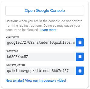
  1. Click the Start Lab button. If you need to pay for the lab, a pop-up opens for you to select your payment method. On the left is a panel populated with the temporary credentials that you must use for this lab.

    Credentials panel

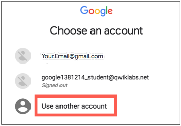
  2. Copy the username, and then click Open Google Console. The lab spins up resources, and then opens another tab that shows the Choose an account page.

    Note: Open the tabs in separate windows, side-by-side.
  3. On the Choose an account page, click Use Another Account. The Sign in page opens.

    Choose an account dialog box with Use Another Account option highlighted

  4. Paste the username that you copied from the Connection Details panel. Then copy and paste the password.

Note: You must use the credentials from the Connection Details panel. Do not use your Google Cloud Skills Boost credentials. If you have your own Google Cloud account, do not use it for this lab (avoids incurring charges).
  1. Click through the subsequent pages:
  • Accept the terms and conditions.
  • Do not add recovery options or two-factor authentication (because this is a temporary account).
  • Do not sign up for free trials.

After a few moments, the Cloud console opens in this tab.

Note: You can view the menu with a list of Google Cloud Products and Services by clicking the Navigation menu at the top-left. Cloud Console Menu

Workbench Instances development environment setup

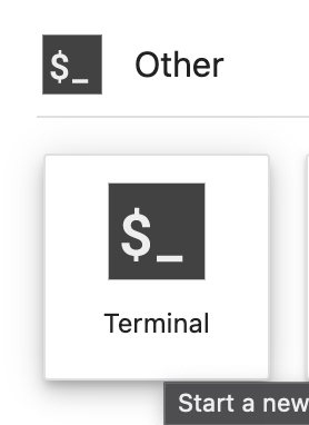
For this lab, you will be running all commands in a terminal from your Instance notebook.

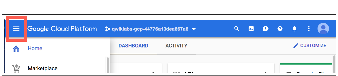
  1. In the Google Cloud console, from the Navigation menu (Navigation menu), select Vertex AI.

  2. Click Enable All Recommended APIs.

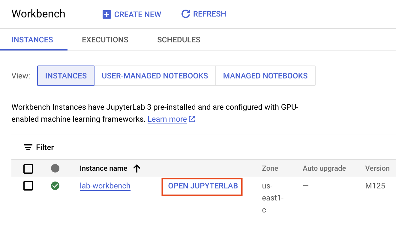
  3. In the Navigation menu, click Workbench.

    At the top of the Workbench page, ensure you are in the Instances view.
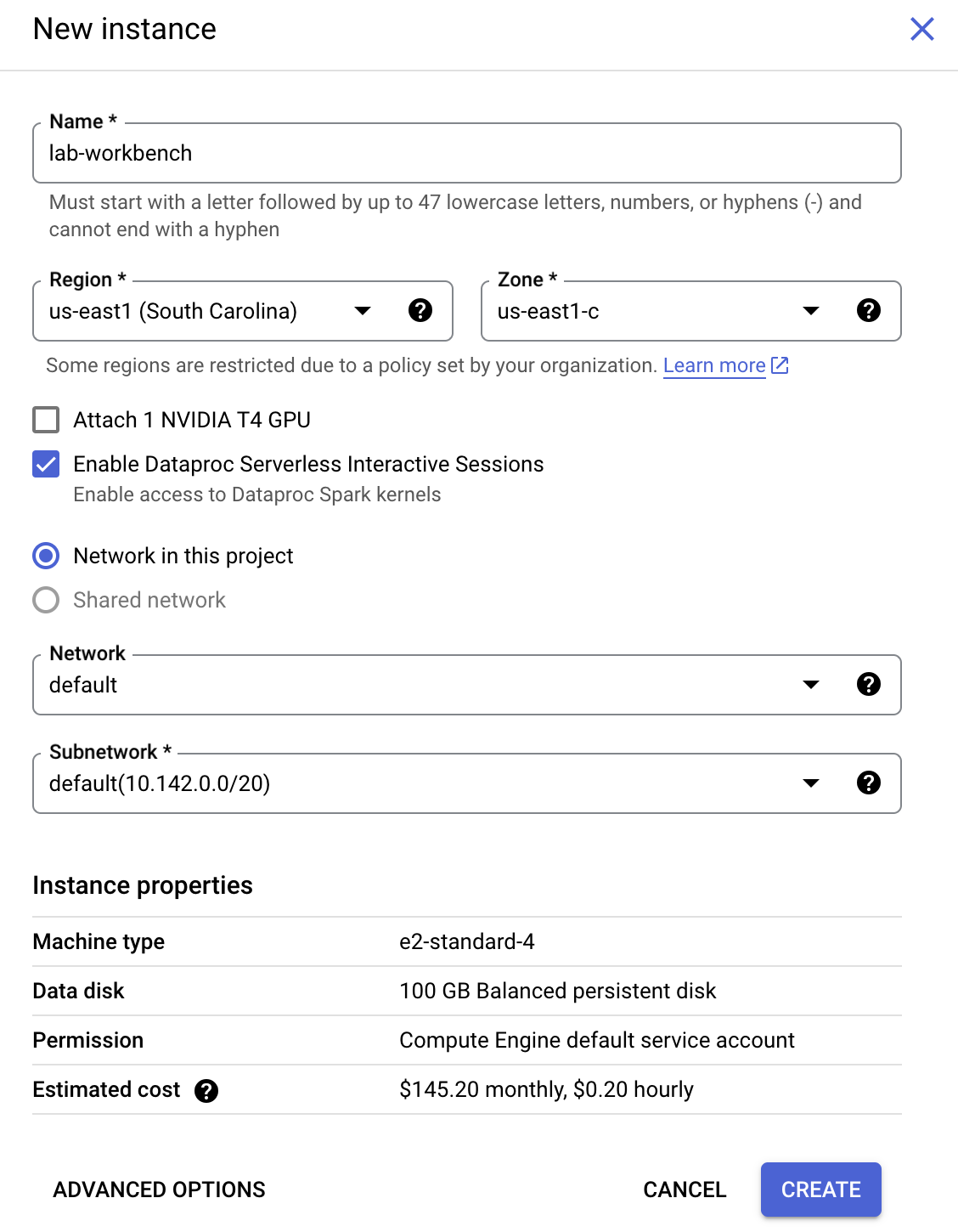
  4. Click add boxCreate New.

  5. Configure the Instance:

    • Name: lab-workbench
    • Region: Set the region to
    • Zone: Set the zone to
    • Advanced Options (Optional): If needed, click "Advanced Options" for further customization (e.g., machine type, disk size).

Create a Vertex AI Workbench instance

  1. Click Create.

This will take a few minutes to create the instance. A green checkmark will appear next to its name when it's ready.

  1. Click Open Jupyterlab next to the instance name to launch the JupyterLab interface. This will open a new tab in your browser.

Workbench Instance Deployed

  1. Next, click Terminal. This will open up a terminal where you can run all the commands in this lab. Open Terminal

Download Code Repository

Next you will download a code repository for use in this lab.

  1. In the terminal you just opened, enter the following:
git clone https://github.com/GoogleCloudPlatform/training-data-analyst cd /home/jupyter/training-data-analyst/quests/dataflow_python/
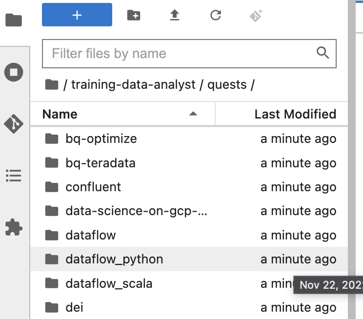
  1. On the left panel of your notebook environment, in the file browser, you will notice the training-data-analyst repo added.

  2. Navigate into the cloned repo /training-data-analyst/quests/dataflow_python/. You will see a folder for each lab, which is further divided into a lab sub-folder with code to be completed by you, and a solution sub-folder with a fully workable example to reference if you get stuck.

Explorer option highlighted in the expanded View menu

Note: To open a file for editing purposes, simply navigate to the file and click on it. This will open the file, where you can add or modify code.

Open the appropriate lab

  • In your terminal, run the following commands to change to the directory you will use for this lab:
# Change directory into the lab cd 5_Streaming_Analytics/lab export BASE_DIR=$(pwd)

Setting up dependencies

Before you can begin editing the actual pipeline code, you need to ensure that you have installed the necessary dependencies.

  1. Execute the following to install the packages you will need to execute your pipeline:
python3 -m pip install -q --upgrade pip setuptools wheel python3 -m pip install apache-beam[gcp]
  1. Ensure that the Dataflow API is enabled:
gcloud services enable dataflow.googleapis.com
  1. Finally, grant the dataflow.worker role to the Compute Engine default service account:
PROJECT_ID=$(gcloud config get-value project) export PROJECT_NUMBER=$(gcloud projects list --filter="$PROJECT_ID" --format="value(PROJECT_NUMBER)") export serviceAccount=""$PROJECT_NUMBER"-compute@developer.gserviceaccount.com"
  1. In the Cloud Console, navigate to IAM & ADMIN > IAM, click on Edit principal icon for Compute Engine default service account.

  2. Add Dataflow Worker as another role and click Save.

Set up the data environment

# Create GCS buckets and BQ dataset cd $BASE_DIR/../.. source create_streaming_sinks.sh # Change to the directory containing the practice version of the code cd $BASE_DIR

Click Check my progress to verify the objective. Set up the data environment

Task 1. Reading from a streaming source

In the previous labs, you used beam.io.ReadFromText to read from Google Cloud Storage. In this lab, instead of Google Cloud Storage, you use Pub/Sub. Pub/Sub is a fully managed real-time messaging service that allows publishers to send messages to a "topic," to which subscribers can subscribe via a "subscription."

The five-point pipeline from the publisher to the subscriber, in which point 2 'Message Storage' and point 3 'Subscription' are highlighted

The pipeline you create subscribes to a topic called my_topic that you just created via create_streaming_sinks.sh script. In a production situation, this topic will often be created by the publishing team. You can view it in the Pub/Sub portion of the console.

  1. In the file explorer, navigate to training-data-analyst/quest/dataflow_python/5_Streaming_Analytics/lab/ and open the streaming_minute_traffic_pipeline.py file.
  • To read from Pub/Sub using Apache Beam’s IO connectors, add a transform to the pipeline which uses the beam.io.ReadFromPubSub() class. This class has attributes for specifying the source topic as well as the timestamp_attribute. By default, this attribute is set to the message publishing time.
Note: Publication time is the time when the Pub/Sub service first receives the message. In systems where there may be a delay between the actual event time and publish time (i.e., late data) and you would like to take this into account, the client code publishing the message needs to set a 'timestamp' metadata attribute on the message and provide the actual event timestamp, since Pub/Sub will not natively know how to extract the event timestamp embedded in the payload. You can see the client code generating the messages you'll use here.

To complete this task:

  • Add a transform that reads from the Pub/Sub topic specified by the input_topic command-line parameter.
  • Then, use the provided function, parse_json with beam.Map to convert each JSON string into a CommonLog instance.
  • Collect the results from this transform into a PCollection of CommonLog instances using with_output_types().
  1. In the first #TODO, add the following code:
beam.io.ReadFromPubSub(input_topic)

Task 2. Window the data

In the previous non-SQL lab, you implemented fixed-time windowing in order to group events by event time into mutually-exclusive windows of fixed size. Do the same thing here with the streaming inputs. Feel free to reference the previous lab's code or the solution if you get stuck.

Window into one-minute windows

To complete this task:

  1. Add a transform to your pipeline that accepts the PCollection of CommonLog data and windows elements into windows of window_duration seconds long, with window_duration as another command-line parameter.
  2. Use the following code to add a transform to your pipeline that windows elements into one-minute windows:
"WindowByMinute" >> beam.WindowInto(beam.window.FixedWindows(60))

Task 3. Aggregate the data

In the previous lab, you used the CountCombineFn() combiner to count the number of events per window. Do the same here.

Count events per window

To complete this task:

  1. Pass the windowed PCollection as input to a transform that counts the number of events per window.
  2. After this, use the provided DoFn, GetTimestampFn, with beam.ParDo to include the window start timestamp.
  3. Use the following code to add a transform to your pipeline that counts the number of events per window:
"CountPerMinute" >> beam.CombineGlobally(CountCombineFn()).without_defaults()

Task 4. Write to BigQuery

This pipeline writes to BigQuery in two separate branches. The first branch writes the aggregated data to BigQuery. The second branch, which has already been authored for you, writes out some metadata regarding each raw event, including the event timestamp and the actual processing timestamp. Both write directly to BigQuery via streaming inserts.

Write aggregated data to BigQuery

Writing to BigQuery has been covered extensively in previous labs, so the basic mechanics will not be covered in depth here.

To complete this task:

  • Create a new command-line parameter called agg_table_name for the table intended to house aggregated data.
  • Add a transfrom as before that writes to BigQuery.
Note: When in a streaming context, beam.io.WriteToBigQuery() does not support write_disposition of WRITE_TRUNCATE in which the table is dropped and recreated. In this example, use WRITE_APPEND.

BigQuery insertion method

beam.io.WriteToBigQuery will default to either streaming inserts for unbounded PCollections or batch file load jobs for bounded PCollections. Streaming inserts can be particularly useful when you want data to show up in aggregations immediately, but does incur extra charges. In streaming use cases where you are OK with periodic batch uploads on the order of every couple minutes, you can specify this behavior via the method keyword argument, and also set the frequency with the triggering_frequency keyword argument. Learn more from the Write data to BigQuery section of the apache_beam.io.gcp.bigquery module documentation.

  • Use the following code to add a transform to your pipeline that writes aggregated data to the BigQuery table.
'WriteAggToBQ' >> beam.io.WriteToBigQuery( agg_table_name, schema=agg_table_schema, create_disposition=beam.io.BigQueryDisposition.CREATE_IF_NEEDED, write_disposition=beam.io.BigQueryDisposition.WRITE_APPEND )

Task 5. Run your pipeline

  • Return to the terminal and execute the following code to run your pipeline:
export PROJECT_ID=$(gcloud config get-value project) export REGION='{{{project_0.default_region|Region}}}' export BUCKET=gs://${PROJECT_ID} export PIPELINE_FOLDER=${BUCKET} export RUNNER=DataflowRunner export PUBSUB_TOPIC=projects/${PROJECT_ID}/topics/my_topic export WINDOW_DURATION=60 export AGGREGATE_TABLE_NAME=${PROJECT_ID}:logs.windowed_traffic export RAW_TABLE_NAME=${PROJECT_ID}:logs.raw python3 streaming_minute_traffic_pipeline.py \ --project=${PROJECT_ID} \ --region=${REGION} \ --staging_location=${PIPELINE_FOLDER}/staging \ --temp_location=${PIPELINE_FOLDER}/temp \ --runner=${RUNNER} \ --input_topic=${PUBSUB_TOPIC} \ --window_duration=${WINDOW_DURATION} \ --agg_table_name=${AGGREGATE_TABLE_NAME} \ --raw_table_name=${RAW_TABLE_NAME} Note: If you get a Dataflow pipeline failed error saying that it is unable to open the pipeline.py file, run the pipeline again and it should run with no issues.

Ensure in the Dataflow UI that it executes successfully without errors. Note that there is no data yet being created and ingested by the pipeline, so it will be running but not processing anything. You will introduce data in the next step.

Click Check my progress to verify the objective. Run your pipeline

Task 6. Generate lag-less streaming input

Because this is a streaming pipeline, it subscribes to the streaming source and will await input; there is none currently. In this section, you generate data with no lag. Actual data will almost invariably contain lag. However, it is instructive to understand lag-less streaming inputs.

The code for this quest includes a script for publishing JSON events using Pub/Sub.

  • To complete this task and start publishing messages, open a new terminal side-by-side with your current one and run the following script. It will keep publishing messages until you kill the script. Make sure you are in the training-data-analyst/quests/dataflow_python folder.
bash generate_streaming_events.sh

Click Check my progress to verify the objective. Generate lag-less streaming input

Examine the results

  1. Wait a couple minutes for the data to start to populate. Then navigate to BigQuery and query the logs.minute_traffic table with the following query:
SELECT timestamp, page_views FROM `logs.windowed_traffic` ORDER BY timestamp ASC

You should see that the number of pageviews hovered around 100 views a minute.

  1. Alternatively, you can use the BigQuery command-line tool as a quick way to confirm results are being written:
bq head logs.raw bq head logs.windowed_traffic
  1. Now, enter the following query:
SELECT UNIX_MILLIS(TIMESTAMP(event_timestamp)) - min_millis.min_event_millis AS event_millis, UNIX_MILLIS(TIMESTAMP(processing_timestamp)) - min_millis.min_event_millis AS processing_millis, user_id, -- added as unique label so we see all the points CAST(UNIX_MILLIS(TIMESTAMP(event_timestamp)) - min_millis.min_event_millis AS STRING) AS label FROM `logs.raw` CROSS JOIN ( SELECT MIN(UNIX_MILLIS(TIMESTAMP(event_timestamp))) AS min_event_millis FROM `logs.raw`) min_millis WHERE event_timestamp IS NOT NULL ORDER BY event_millis ASC

This query illustrates the gap between event time and processing time. However, it can be hard to see the big picture by looking at just the raw tabular data. We will use Looker Studio, a lightweight data visualization and BI engine.

  1. To enable Looker Studio:
  • Visit Looker Studio.
  • Click Create in the upper left.
  • Click Report.
  • Select Country name and enter a Company name. Check the checkbox to acknowledge you have read and agree to the Looker Studio Additional Terms, then click Continue.
  • Select "No" to all options, then click Continue.
  • Return to the BigQuery UI.
  1. In the BigQuery UI, click on the Open in dropdown and choose Looker Studio.

This will open a new window.

  1. Click Get Started.

Notice that default visualizations are created for the data.

  1. To remove the default visualizations, right-click on each, and select Delete.

  2. Click Add a chart on the top menu bar.

  3. Select the Scatter chart type.

  4. In the Data column of the panel on the right hand side, set the following values:

  • Dimension: label
  • Metric X: event_millis
  • Metric Y: processing_millis

The chart will transform to be a scatterplot, where all points are on the diagonal. This is because in the streaming data currently being generated, events are processed immediately after they were generated — there was no lag. If you started the data generation script quickly, i.e. before the Dataflow job was fully up and running, you may see a hockey stick, as there were messages queuing in Pub/Sub that were all processed more or less at once.

But in the real world, lag is something that pipelines need to cope with.

A scatterplot wherein all points are diagonal

Task 7. Introduce lag to streaming input

The streaming event script is capable of generating events with simulated lag.

This represents scenarios where there is a time delay between when the events are generated and published to Pub/Sub, for example when a mobile client goes into offline mode if a user has no service, but events are collected on the device and all published at once when the device is back online.

Generate streaming input with lag

  1. First, close the Looker Studio window.

  2. Then, to turn on lag, return to the terminal and stop the running script using CTRL+C.

  3. Then, run the following:

bash generate_streaming_events.sh true

Examine the results

  • Return to the BigQuery UI, rerun the query, and then recreate the Looker Studio view as before. The new data that arrive, which should appear on the right side of the chart, should no longer be perfect; instead, some will appear above the diagonal, indicating that they were processed after the events transpired.

Chart Type: Scatter

  • Dimension: label
  • Metric X: event_millis
  • Metric Y: processing_millis

A scatter chart wherein some data points are above the diagonal line

End your lab

When you have completed your lab, click End Lab. Google Cloud Skills Boost removes the resources you’ve used and cleans the account for you.

You will be given an opportunity to rate the lab experience. Select the applicable number of stars, type a comment, and then click Submit.

The number of stars indicates the following:

  • 1 star = Very dissatisfied
  • 2 stars = Dissatisfied
  • 3 stars = Neutral
  • 4 stars = Satisfied
  • 5 stars = Very satisfied

You can close the dialog box if you don't want to provide feedback.

For feedback, suggestions, or corrections, please use the Support tab.

Copyright 2022 Google LLC All rights reserved. Google and the Google logo are trademarks of Google LLC. All other company and product names may be trademarks of the respective companies with which they are associated.

准备工作

  1. 实验会创建一个 Google Cloud 项目和一些资源,供您使用限定的一段时间
  2. 实验有时间限制,并且没有暂停功能。如果您中途结束实验,则必须重新开始。
  3. 在屏幕左上角,点击开始实验即可开始

使用无痕浏览模式

  1. 复制系统为实验提供的用户名密码
  2. 在无痕浏览模式下,点击打开控制台

登录控制台

  1. 使用您的实验凭证登录。使用其他凭证可能会导致错误或产生费用。
  2. 接受条款,并跳过恢复资源页面
  3. 除非您已完成此实验或想要重新开始,否则请勿点击结束实验,因为点击后系统会清除您的工作并移除该项目

此内容目前不可用

一旦可用,我们会通过电子邮件告知您

太好了!

一旦可用,我们会通过电子邮件告知您

一次一个实验

确认结束所有现有实验并开始此实验

使用无痕浏览模式运行实验

请使用无痕模式或无痕式浏览器窗口运行此实验。这可以避免您的个人账号与学生账号之间发生冲突,这种冲突可能导致您的个人账号产生额外费用。