Overview

BigQuery is Google's fully managed, NoOps, low cost analytics database. With BigQuery you can query terabytes and terabytes of data without having any infrastructure to manage, or needing a database administrator. BigQuery uses SQL and can take advantage of the pay-as-you-go model. BigQuery allows you to focus on analyzing data to find meaningful insights.

BigQuery Machine Learning (BQML, product in beta) is a new feature in BigQuery where data analysts can create, train, evaluate, and predict with machine learning models with minimal coding.

In this lab, you will explore millions of New York City yellow taxi cab trips available in a BigQuery public dataset. Then you will create a machine learning model inside of BigQuery to predict the fare of the cab ride given your model inputs. Lastly, you will evaluate the performance of your model and make predictions.

Objectives

In this lab, you will learn how to perform the following tasks:

• Use BigQuery to find public datasets.
• Query and explore the public taxi cab dataset.
• Create a training and evaluation dataset to be used for batch prediction.
• Create a forecasting (linear regression) model in BQML.
• Evaluate the performance of your machine learning model.

What you'll need

• A Google Cloud Platform Project.
• A Browser, such as Google Chrome or Mozilla Firefox.

Setup and requirements

For each lab, you get a new Google Cloud project and set of resources for a fixed time at no cost.

1. Sign in to Google Skills using an incognito window.

2. Note the lab's access time (for example, 1:15:00), and make sure you can finish within that time. There is no pause feature. You can restart if needed, but you have to start at the beginning.

3. When ready, click Start lab.

4. Note your lab credentials (Username and Password). You will use them to sign in to the Google Cloud Console.

5. Click Open Google Console.

6. Click Use another account and copy/paste credentials for this lab into the prompts. If you use other credentials, you'll receive errors or incur charges.

7. Accept the terms and skip the recovery resource page.

Open BigQuery Console

1. In the Google Cloud Console, select Navigation menu > BigQuery.

The Welcome to BigQuery in the Cloud Console message box opens. This message box provides a link to the quickstart guide and lists UI updates.

2. Click Done.

Task 1. Explore NYC taxi cab data

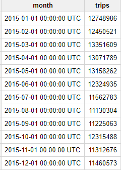
Question: How many trips did Yellow taxis take each month in 2015?

1. Add the following query in the SQLquery editor field:

2. Then click Run.

The result is output as follows.

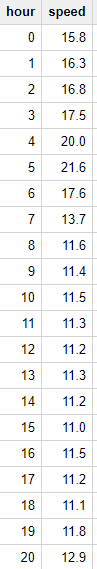
Question: What was the average speed of Yellow taxi trips in 2015?

3. Replace the previous query with the following, and then click Run:

The result is output as follows.

During the day, the average speed is around 11-12 MPH; but at 5:00 AM the average speed almost doubles to 21 MPH. Intuitively this makes sense since there is likely less traffic on the road at 5:00 AM.

Task 2. Identify an objective

You will now create a machine learning model in BigQuery to predict the price of a cab ride in New York city given the historical dataset of trips and trip data. Predicting the fare before the ride could be very useful for trip planning for both the rider and the taxi agency.

Select features and create your training dataset

The New York City Yellow Cab dataset is a public dataset provided by the city and has been loaded into BigQuery for your exploration. Browse the complete list of fields and then preview the dataset to find useful features that will help a machine learning model understand the relationship between data about historical cab rides and the price of the fare.

Your team decides to test whether these below fields are good inputs to your fare forecasting model:

• Tolls Amount
• Fare Amount
• Hour of Day
• Pick up address
• Drop off address
• Number of passengers

1. Replace the query with the following:

Note a few things about the query:

• The main part of the query is at the bottom: (SELECT * from taxitrips).
• taxitrips does the bulk of the extraction for the NYC dataset, with the SELECT containing your training features and label.
• The WHERE removes data that you don't want to train on.
• The WHERE also includes a sampling clause to pick up only 1/1000th of the data.
• We define a variable called TRAIN so that you can quickly build an independent EVAL set.

2. Then click Run.

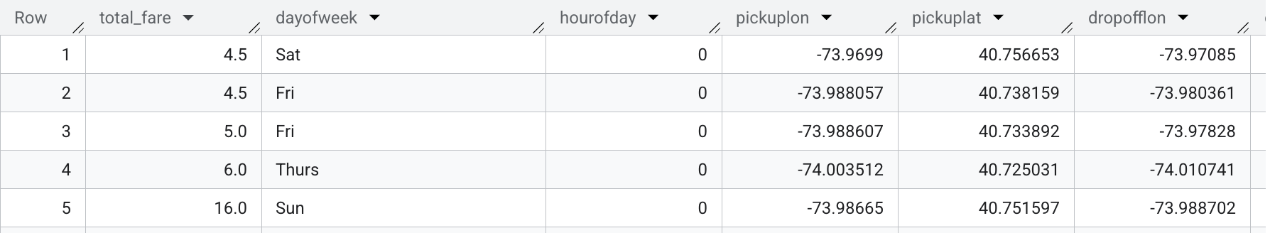
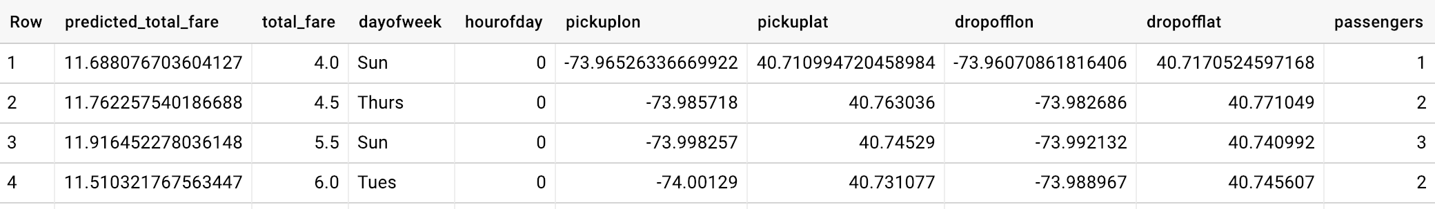
The sample results are as indicated below.

Question: What is the label (correct answer)?

In this case, total_fare is the label (that we will be predicting). You created this field out of tolls_amount and fare_amount, so you could ignore customer tips as part of the model, as they are discretionary.

Task 3. Create a BigQuery dataset to store models

Next, create a new BigQuery dataset which will also store your ML models.

1. In the Explorer pane, click the View actions icon next to your project ID. Click Create datatset.

2. In the Create dataset dialog:

• For Dataset ID, type taxi.
• Leave the other values at their defaults.

3. Click Create dataset.

Task 4. Select a BQML model type and specify options

Now that you have your initial features selected, you are now ready to create your first ML model in BigQuery.

There are the two model types to choose from.

Question: Which model type should you choose? Since you are predicting a numeric value (cab fare) you want to use linear regression.

1. Enter the following query to create a model and specify model options, replacing -- paste the previous training dataset query here with the training dataset query you created earlier (omitting the #standardSQL line):

2. Next, click Run to train your model.

Wait for the model to train (about 5 - 10 minutes).

After your model is trained, you will see the result This statement created a new model named <Project-ID>:taxi.taxifare_model which indicates that your model has been successfully trained.

Look inside your taxi dataset and confirm taxifare_model now appears.

Next, you will evaluate the performance of the model against new unseen evaluation data.

Task 5. Evaluate classification model performance

Select your performance criteria

For linear regression models, you want to use a loss metric like Root Mean Squared Error. You want to keep training and improving the model until it has the lowest RMSE.

1. In BQML, mean_squared_error is simply a queryable field when evaluating your trained ML model. Simply add a SQRT() to get RMSE.

2. Now that training is complete, you can evaluate how well the model performs with this query using ML.EVALUATE:

You are now evaluating the model against a different set of taxi cab trips with your params.EVAL filter.

After the model runs, review your model results (your model RMSE value will vary slightly).

After evaluating your model you get a RMSE of $9.47.

Knowing whether or not this loss metric is acceptable to productionalize your model is entirely dependent on your benchmark criteria, which is set before model training begins. Benchmarking is establishing a minimum level of model performance and accuracy that is acceptable.

Task 6. Compare training and evaluation loss

You want to make sure that you aren't overfitting your model to your data. Overfitting your model will make it perform worse on new, unseen data.

1. You can compare the training loss to the evaluation loss with ML.TRAINING_INFO:

This will select all the information from each iteration of the model training. It will include the training iteration number, the training loss, and the evaluation loss.

To compare training and evaluation loss, let's explore the difference in the loss curves visually.

2. Click on Open in > Looker Studio in the BigQuery Cloud Console. This will open Data Studio with the data from your query connected as an input source.

3. When prompted, click the Get Started button.

4. Select Authorize, when asked if Google Data Studio can access your data.

5. Click on Get Started and acknowledge the Terms of Service. Click Accept.

6. Select No, thanks for all in preferences and click Done.

7. Refresh the tab to load the data.

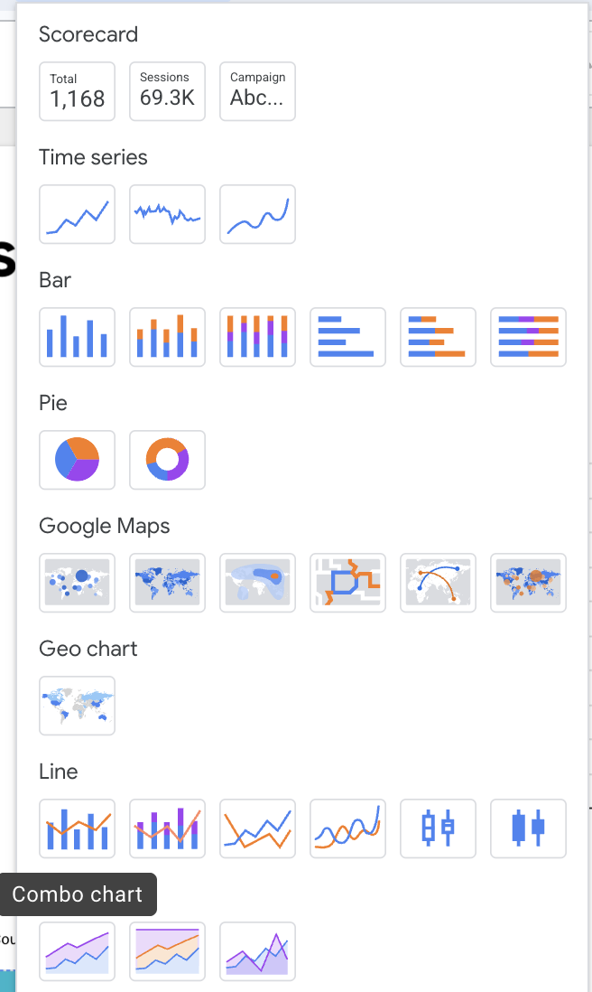
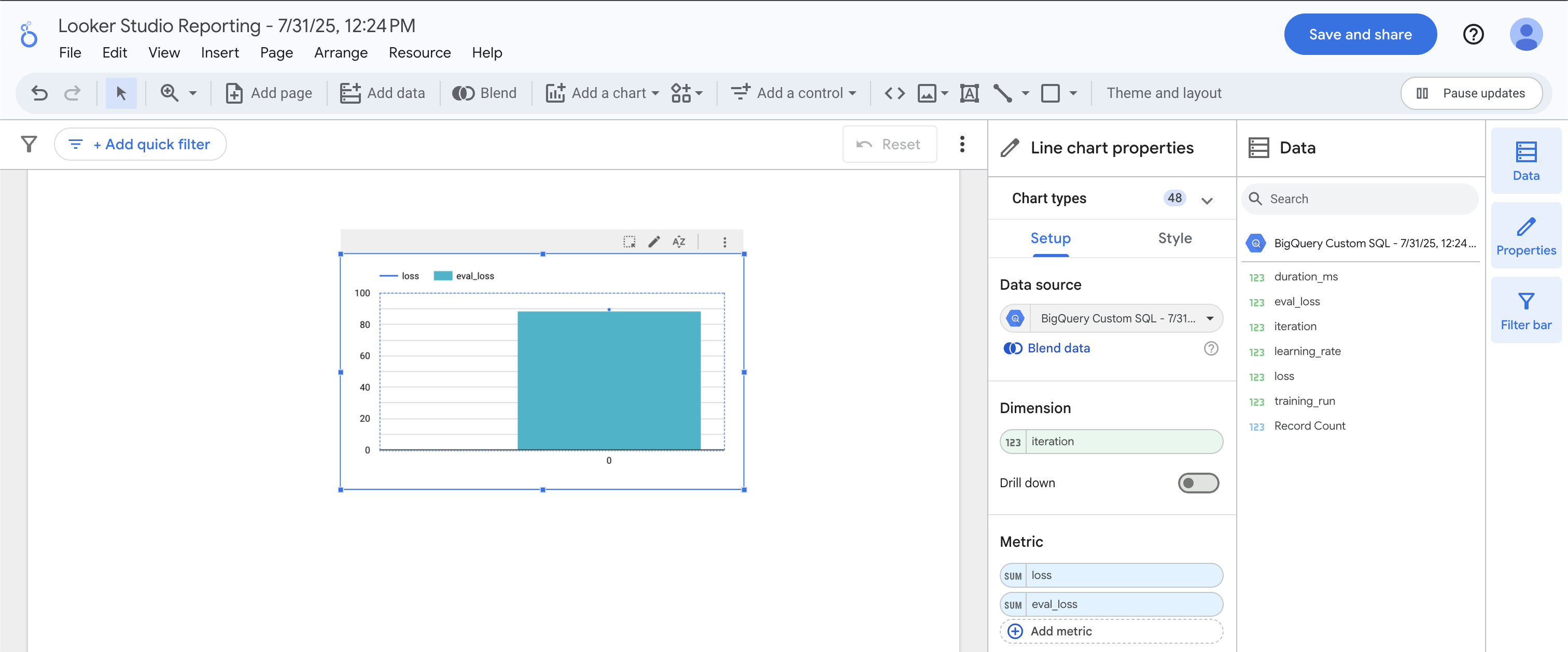
8. Once in Looker Studio, click on the Add Chart > Combo Chart icon.

9. Under Dimension, drag over iteration. Under Metric, drag over both loss and eval_loss. You should get a chart that features a line chart superimposed over a bar chart.

The training loss matches the evaluation loss nearly identically, which indicates that we are not overfitting the model.

Excellent! Let's move on to prediction.

Task 7. Predict a taxi fare amount

• Next, you will write a query to use your new model to make predictions:

Now you will see the model's predictions for taxi fares alongside the actual fares and other features for those rides.

Additional information

Tip: Add warm_start = true to your model options if you are retraining new data on an existing model for faster training times. Note that you cannot change the feature columns (this would necessitate a new model).

Other datasets to explore

You can use the Chicago taxi trips dataset to bring in the bigquery-public-data project if you want to explore modeling on other datasets like forecasting fares for Chicago taxi trips.

Congratulations!

In this lab, you have successfully built an ML model in BigQuery to forecast taxi cab fare for New York City cabs.

End your lab

When you have completed your lab, click End Lab. Google Skills removes the resources you’ve used and cleans the account for you.

You will be given an opportunity to rate the lab experience. Select the applicable number of stars, type a comment, and then click Submit.

The number of stars indicates the following:

• 1 star = Very dissatisfied
• 2 stars = Dissatisfied
• 3 stars = Neutral
• 4 stars = Satisfied
• 5 stars = Very satisfied

You can close the dialog box if you don't want to provide feedback.

For feedback, suggestions, or corrections, please use the Support tab.

Copyright 2026 Google LLC All rights reserved. Google and the Google logo are trademarks of Google LLC. All other company and product names may be trademarks of the respective companies with which they are associated.